Filtering samples and features with singlecellutils
Jens Preussner
2019-02-07
Source:vignettes/singlecellutils-filtering.Rmd
singlecellutils-filtering.RmdThis vignette will teach you how to use methods from singlecellutils to detect and filter low quality samples and exclude features that are lowly expressed. Methods from singlecellutils are enabled for piping (using magrittrs pipe operator) and allow you to write code that is easily understandable.
Load an example data set - 1k Brain cells
Throughout this vignette, you’ll use the 1k Brain Cells dataset from 10xgenomics.com. It ships with singlecellutils and is already preprocessed as a SingleCellExperiment data object from the SingleCellExperiment package. Just load the object like below and you’re good to go:
Low quality sample filtering
Samples of low quality are typically associated with the detection of only a few features (e.g. genes) or have generated only a low number of sequencing reads due to deteriorated DNA. During preprocessing of dataset loaded above, we also ran the calculateQCMetrics() function from the scater package, that adds such important quality criteria to the colData slot of the neuron_1k_v3 object. Take a quick look to get a feeling for the information that is available:
head(SummarizedExperiment::colData(neuron_1k_v3))
#> DataFrame with 6 rows and 9 columns
#>                    is_cell_control total_features_by_umi
#>                          <logical>             <integer>
#> AAACGAATCAAAGCCT-1           FALSE                   417
#> AAACGCTGTAATGTGA-1           FALSE                  2744
#> AAACGCTGTCCTGGGT-1           FALSE                  3603
#> AAAGAACCAGGACATG-1           FALSE                  2386
#> AAAGGTACACACGGTC-1           FALSE                  4748
#> AAAGTCCAGTCACTAC-1           FALSE                  5104
#>                    log10_total_features_by_umi total_umi  log10_total_umi
#>                                      <numeric> <numeric>        <numeric>
#> AAACGAATCAAAGCCT-1            2.62117628177504      1023 3.01029995663981
#> AAACGCTGTAATGTGA-1            3.43854234878611      7210 3.85799549556092
#> AAACGCTGTCCTGGGT-1            3.55678478230703      9883 3.99493273673004
#> AAAGAACCAGGACATG-1            3.37785241900675      5290 3.72353776153206
#> AAAGGTACACACGGTC-1            3.67660216958202     18676 4.27130711878496
#> AAAGTCCAGTCACTAC-1            3.70799574642293     20196 4.30528686547613
#>                    pct_umi_in_top_50_features pct_umi_in_top_100_features
#>                                     <numeric>                   <numeric>
#> AAACGAATCAAAGCCT-1           64.1251221896383            69.0127077223851
#> AAACGCTGTAATGTGA-1           29.9583911234397            38.4466019417476
#> AAACGCTGTCCTGGGT-1           22.2908023879389            29.8391176768188
#> AAAGAACCAGGACATG-1           22.5141776937618            30.4914933837429
#> AAAGGTACACACGGTC-1           22.4780466909402            34.2150353394731
#> AAAGTCCAGTCACTAC-1           23.9255298078827            32.9570211923153
#>                    pct_umi_in_top_200_features pct_umi_in_top_500_features
#>                                      <numeric>                   <numeric>
#> AAACGAATCAAAGCCT-1            78.7878787878788                         100
#> AAACGCTGTAATGTGA-1            47.3509015256588            61.5811373092926
#> AAACGCTGTCCTGGGT-1            39.2492158251543            53.8298087625215
#> AAAGAACCAGGACATG-1            40.1701323251418            56.9754253308129
#> AAAGGTACACACGGTC-1            44.8704219318912            58.2512315270936
#> AAAGTCCAGTCACTAC-1            43.1867696573579             56.387403446227
You’re particularly interested in the total_features_by_umi column, whose values count the number of detected features, and in the total_umi column, whose values count the number of unique molecular identifiers (UMI) associated with each sample.
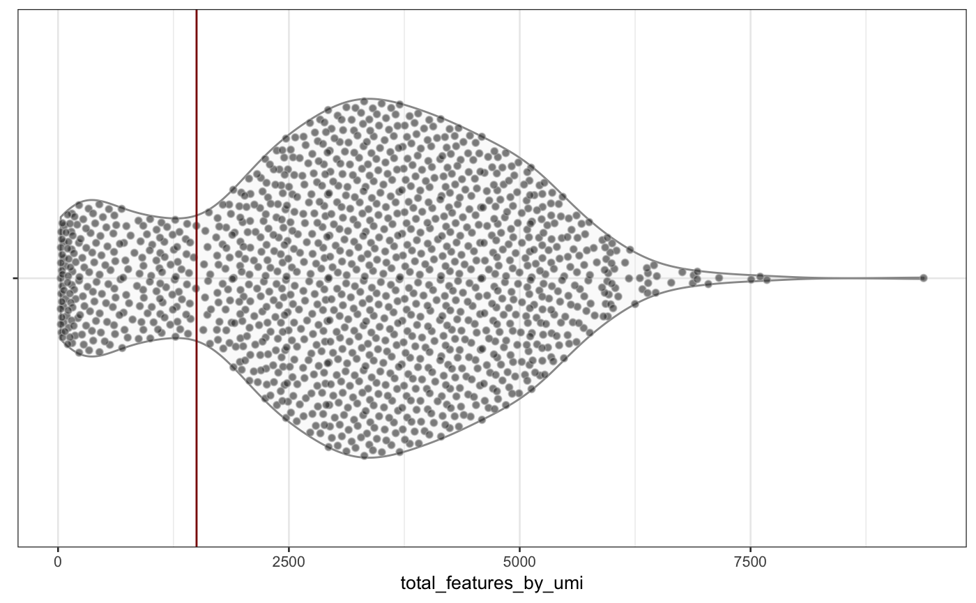
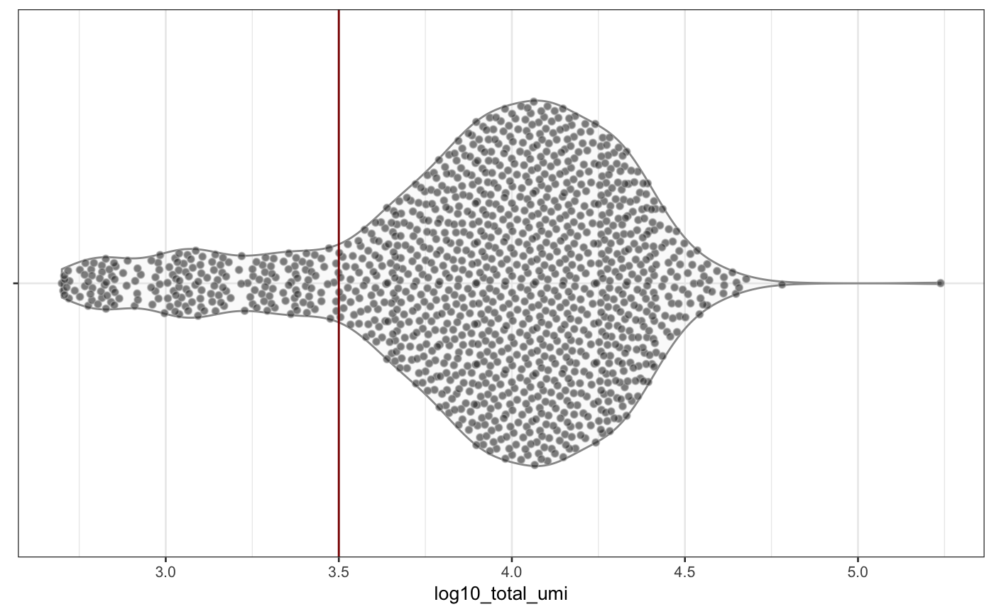
Let’s check how those two quality criteria distribute, by plotting a violin plot, where each sample is represented by a dot:
scater::plotColData(neuron_1k_v3, y = "total_features_by_umi")
scater::plotColData(neuron_1k_v3, y = "log10_total_umi")

Distribution of total_features_by_umi and total_umi (log-scaled) across all samples in the neuron_1k_v3 dataset.
From the figure above, you can see that roughly 1500 features are detected in the vast majority of samples. Further, most of the cells are associated with \(10^{3.5}\) (thats slightly more than 3100) or more distinct UMIs. Samples below those values (or left of the red vertical lines) are potentially outliers and could be removed before downstream analysis1.
The
singlecellutilspackage adopts the approach of the genefilter package to filter samples and features. The idea is to combine output from multiple filter functions, each returningTRUEorFALSEfor every sample/feature, indicating if the sample/feature should be filtered out or not. However,singlecellutilsextends the functionality of genefilter to allow OR conjunctions between filters as well.
Create two sample filters, using the kOverA function from genefilter and the EpOverA function from singlecellutils:
sample_filter <- list("genefilter::kOverA" = list(k = 1500, A = 1),
"singlecellutils::EpOverA" = list(A = 3100))Explanation: genefilter::kOverA is a filter function that returns TRUE, if k inspected values are above a value of A. In our case, k = 1500 features have to exceed a UMI count of A = 1, indicating expression. singlecellutils::EpOverA is a filter function, that returns TRUE if the aggregate of values is above A. In our case, samples have to exceed an aggregated UMI count of A = 3100.
For example, after a call to
the neuron_1k_v3 object contains 601 remaining samples. If you would like to combine filters with an OR conjunction use the tolerate argument of filter_samples:
neuron_1k_v3 %<>%
  singlecellutils::filter_samples(sample_filter, exprs_values = "umi", tolerate = 1)
In this case, 1108 high quality samples remain.
Filtering lowly expressed genes
Similar to low quality samples, lowly expressed features can also obfuscate downstream analysis (e.g. dimension reduction or clustering) and should be removed as well. Again, take a quick look at the output of the calculateQCMetrics() function, this time for feature-based quality measures:
head(SummarizedExperiment::rowData(neuron_1k_v3))
#> DataFrame with 6 rows and 10 columns
#>                               gene_id   gene_name         feature
#>                           <character> <character>     <character>
#> ENSMUSG00000051951 ENSMUSG00000051951        Xkr4 Gene Expression
#> ENSMUSG00000089699 ENSMUSG00000089699      Gm1992 Gene Expression
#> ENSMUSG00000102343 ENSMUSG00000102343     Gm37381 Gene Expression
#> ENSMUSG00000025900 ENSMUSG00000025900         Rp1 Gene Expression
#> ENSMUSG00000025902 ENSMUSG00000025902       Sox17 Gene Expression
#> ENSMUSG00000104328 ENSMUSG00000104328     Gm37323 Gene Expression
#>                    is_feature_control             mean_umi
#>                             <logical>            <numeric>
#> ENSMUSG00000051951              FALSE    0.116064565718678
#> ENSMUSG00000089699              FALSE 0.000768639508070715
#> ENSMUSG00000102343              FALSE                    0
#> ENSMUSG00000025900              FALSE  0.00153727901614143
#> ENSMUSG00000025902              FALSE   0.0653343581860108
#> ENSMUSG00000104328              FALSE 0.000768639508070715
#>                          log10_mean_umi n_cells_by_umi pct_dropout_by_umi
#>                               <numeric>      <integer>          <numeric>
#> ENSMUSG00000051951   0.0476893198024886            120   90.7763259031514
#> ENSMUSG00000089699 0.000333687670586935              1   99.9231360491929
#> ENSMUSG00000102343                    0              0                100
#> ENSMUSG00000025900 0.000667119150998434              2   99.8462720983859
#> ENSMUSG00000025902   0.0274859337142017             11   99.1544965411222
#> ENSMUSG00000104328 0.000333687670586935              1   99.9231360491929
#>                    total_umi   log10_total_umi
#>                    <numeric>         <numeric>
#> ENSMUSG00000051951       151  2.18184358794477
#> ENSMUSG00000089699         1 0.301029995663981
#> ENSMUSG00000102343         0                 0
#> ENSMUSG00000025900         2 0.477121254719662
#> ENSMUSG00000025902        85  1.93449845124357
#> ENSMUSG00000104328         1 0.301029995663981
Maybe you’re particularly interested in the mean_umi column, whose values represent the mean UMI count of the feature across all samples, and in the n_cells_by_umi column, whose values count the number of samples that express the feature.
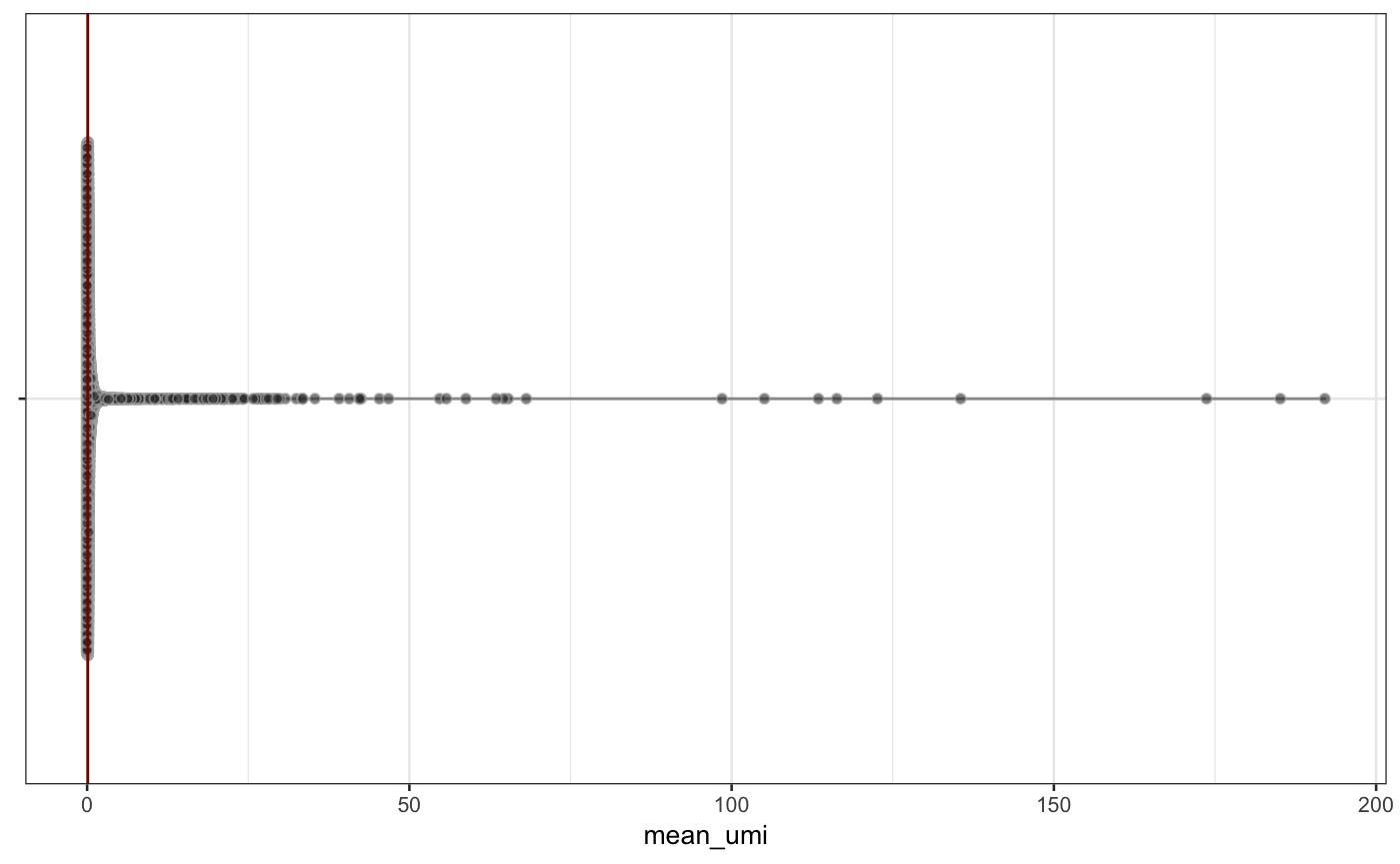
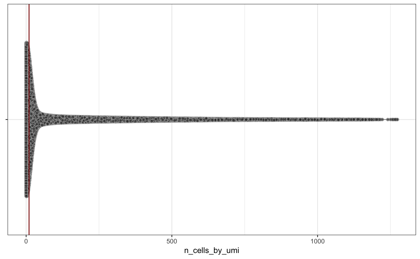
Let’s check how those two quality criteria distribute, by plotting a violin plot, where each feature is represented by a dot:
scater::plotRowData(neuron_1k_v3, y = "mean_umi")
scater::plotRowData(neuron_1k_v3, y = "n_cells_by_umi")

Distribution of mean_umi and n_cells_by_umi across all features in the neuron_1k_v3 dataset.
From the figure above, you can see that most features are expressed at very low levels (the red bar indicates a mean of 0.1) and only in a fraction of samples (the red bar indicates 20 samples). We will demonstrate feature filtering using two filter functions from singlecellutils and genefilter:
feature_filter <- list("singlecellutils::MeanOverA" = list(A = 0.1),
"genefilter::kOverA" = list(k = 10, A = 1))Explanation: singlecellutils::MeanOverA is a filter function that returns TRUE, if the mean of the inspected values are above a value of A. In our case, the mean UMI count of a feature has to be above A = 0.1 for the feature to remain in the dataset. genefilter::kOverA is a filter function that returns TRUE, if k inspected values are above a value of A. In our case, features have to be expressed in at least k = 10 samples.
For example, after a call to
the neuron_1k_v3 object contains 9237 remaining features. If you would like to combine filters with an OR conjunction use the tolerate argument of filter_features:
neuron_1k_v3 %<>%
  singlecellutils::filter_features(feature_filter, exprs_values = "umi", tolerate = 1)
In this case, 10173 features remain in the dataset.
Using pipes to filter samples and genes
The examples showing sample and feature filtering from above can easily be combined into one pipeline. This will reduce the amount of code you’ll have to write, enhances visibility of what functions are applied to the neuron_1k_v3 object and normally speeds up your analysis as well. Here we go:
neuron_1k_v3 %<>%
  singlecellutils::filter_samples(list("genefilter::kOverA" = list(k = 1500, A = 1),
                                       "singlecellutils::EpOverA" = list(A = 3100)),
                                  exprs_values = "umi",
                                  tolerate = 1) %>%
  singlecellutils::filter_features(list("singlecellutils::MeanOverA" = list(A = 0.1),
                                        "genefilter::kOverA" = list(k = 10, A = 1)),
                                   exprs_values = "umi",
                                   tolerate = 1)
Using only two lines, the final object is filtered for low quality samples and lowly expressed features and now contains data from 10234 features measured across 1108 samples. Happy downstream analysis ;-)