Dimension reduction and clustering with singlecellutils
Jens Preussner
2019-02-07
Source:vignettes/singlecellutils-dimensionreduction.Rmd
singlecellutils-dimensionreduction.RmdThis vignette will teach you how to use methods from singlecellutils to perform dimension reduction and clustering of samples. Methods from singlecellutils are enabled for piping (using magrittrs pipe operator) and allow you to write code that is easily understandable.
Load an example data set - 1k Brain cells
Throughout this vignette, you’ll use the 1k Brain Cells dataset from 10xgenomics.com. It ships with singlecellutils and is already preprocessed as a SingleCellExperiment data object from the SingleCellExperiment package. Here, we’ll load the object and perform filtering as described in the Filtering samples and features with singlecellutils vignette:
data("neuron_1k_v3", package = "singlecellutils")

neuron_1k_v3 %<>%
  singlecellutils::filter_samples(list("genefilter::kOverA" = list(k = 1500, A = 1),
                                       "singlecellutils::EpOverA" = list(A = 3100)),
                                  exprs_values = "umi",
                                  tolerate = 1) %>%
  singlecellutils::filter_features(list("singlecellutils::MeanOverA" = list(A = 0.1),
                                        "genefilter::kOverA" = list(k = 10, A = 1)),
                                   exprs_values = "umi",
                                   tolerate = 1) %>%
  scater::calculateQCMetrics(exprs_values = "umi")
Normalize the expression using scran and scater
A typical step after filtering is normalization. Here, we’ll rely on a quick and simple calculation of cell-specific size factors using the simpleSumFactors function from the scran package. The function adds the size factors to the sizeFactors-slot in neuron_1k_v3, which is picked up by scater’s normalize function:
Performing dimension reduction using UMAP
UMAP (Uniform Manifold Approximation and Projection) is a novel manifold learning technique for dimension reduction. […] The UMAP algorithm is competitive with t-SNE for visualization quality, and arguably preserves more of the global structure with superior run time performance. Furthermore, UMAP has no computational restrictions on embedding dimension, making it viable as a general purpose dimension reduction technique for machine learning.
from the UMAP paper abstract
Two parameters determine UMAPs performance:
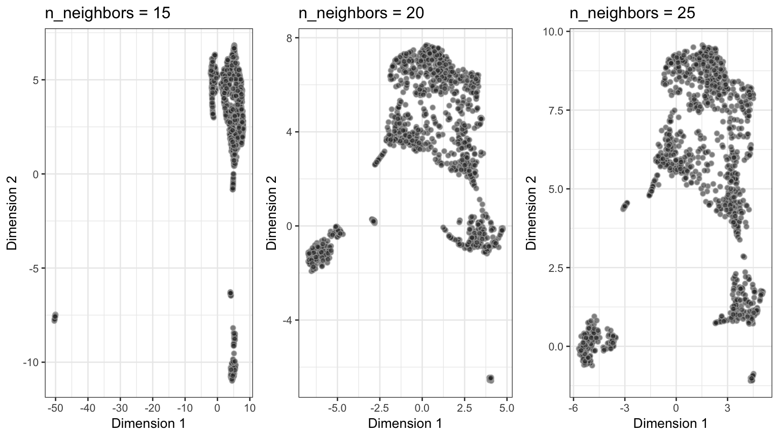
The number of neighboring points determines how much of the global structure is being preserved at the loss of local structure. Larger values preserve more of the global structure and values in the range of 5 to 50 are mostly fine, with 10-15 being sensible defaults.
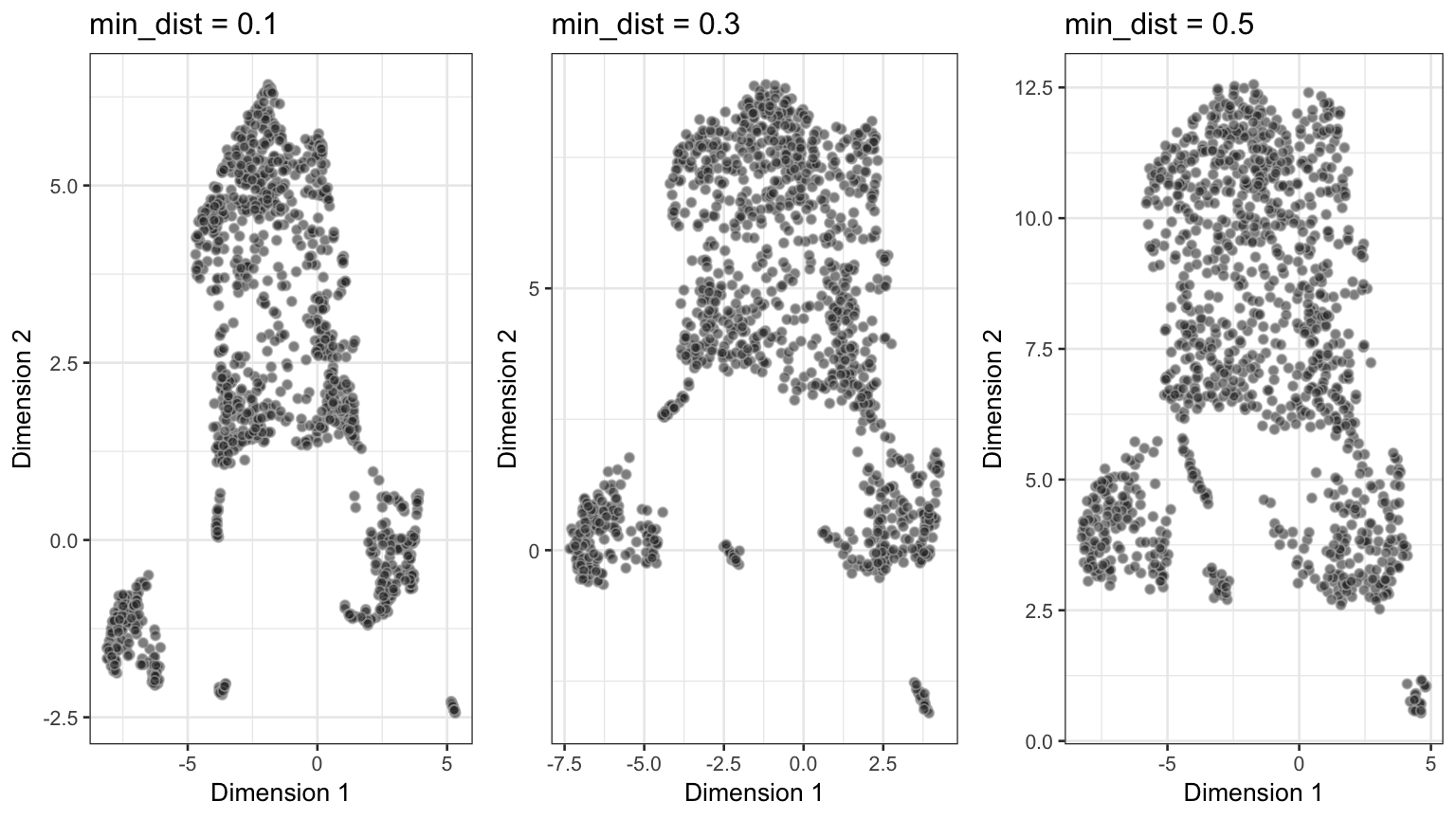
The minimum distance controls how tightly the embedding is allowed to compress points together. Larger values ensure embedded points are more evenly distributed, while smaller values allow the algorithm to optimise more accurately with regard to local structure. Sensible values are in the range 0.001 to 0.5, with 0.1 being a reasonable default.
We’ll first explore, how different values of one of those two parameters change the embedding, when keeping the other value fixed:

Performance of UMAP across differen values of n_neighbors.

Performance of UMAP across differen values of min_dist.
As we can see from above, a value of 20 for n_neighbors should be chosen at minimum, whereas the min_dist should not exceed 0.1 to permit reliable identification of subclusters.
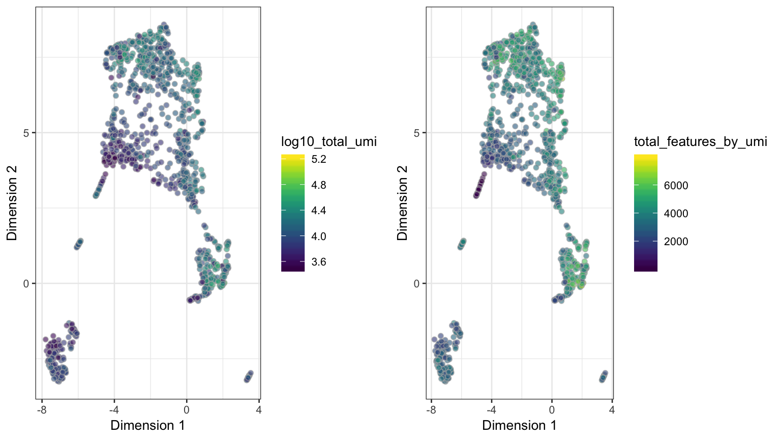
We can now use UMAP and visualize the resulting dimension reduction in several ways:
neuron_1k_v3 %<>%
singlecellutils::reduce_dimension(flavor = "umap",
exprs_values = "logcounts",
n_neighbors = 20L,
min_dist = 0.1,
seed = 2304)and visualize the dimension reduction with different quality criteria (see Section visualization for source code examples):

UMAP dimension reduction on the neuron_1k_v3 dataset, using n_neighbors = 20 and min_dist = 0.1 as input parameters.
Clustering samples using HDBSCAN
Hierarchical Density-Based Spatial Clustering of Applications with Noise (HDBSCAN)1, is a new density-based clustering algorithm that extends DBSCAN2 by converting it into a hierarchical clustering algorithm, and then using a technique to extract a flat clustering based in the stability of clusters. This allows HDBSCAN to find clusters of varying densities (unlike DBSCAN), and be more robust to parameters.
neuron_1k_v3 %<>%
singlecellutils::add_clustering(flavor = "hdbscan",
use_dimred = "umap",
column = ".clustering_911",
min_samples = 9L,
min_cluster_size = 11L)Visualization of dimension reduction and clustering
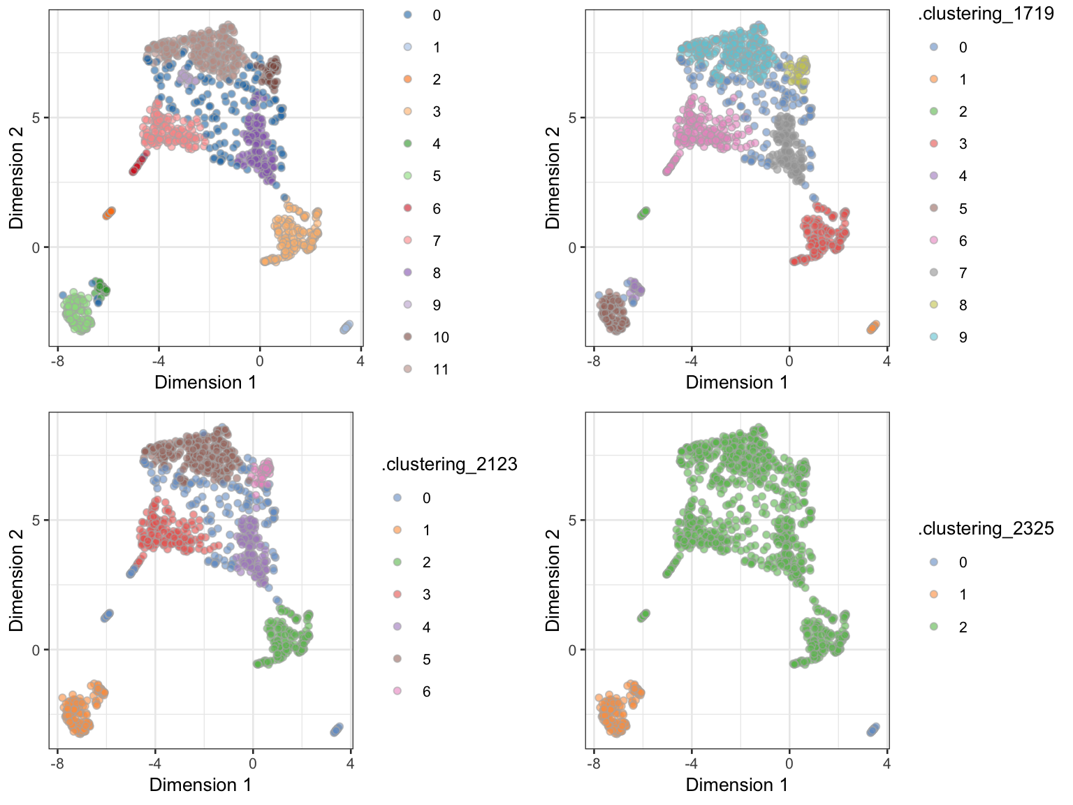
Visualization of different clusterings (e.g. different parameters) can be performed with functions from the scater package:
hdbscan_p1 <- scater::plotReducedDim(neuron_1k_v3, use_dimred = "umap", colour_by = ".clustering_911", add_ticks = FALSE)
hdbscan_p2 <- scater::plotReducedDim(neuron_1k_v3, use_dimred = "umap", colour_by = ".clustering_1719", add_ticks = FALSE)
hdbscan_p3 <- scater::plotReducedDim(neuron_1k_v3, use_dimred = "umap", colour_by = ".clustering_2123", add_ticks = FALSE)
hdbscan_p4 <- scater::plotReducedDim(neuron_1k_v3, use_dimred = "umap", colour_by = ".clustering_2325", add_ticks = FALSE)
gridExtra::grid.arrange(hdbscan_p1, hdbscan_p2, hdbscan_p3, hdbscan_p4, nrow = 2)
UMAP dimension reduction on the neuron_1k_v3 dataset, coloured by different HDBSCAN clusterings.
Using pipes to reduce dimension and perform clustering
The code snippets from above for normalization, dimension reduction and clustering can easily be combined into one pipeline. This will reduce the amount of code you’ll have to write, enhances visibility of what functions are applied to the neuron_1k_v3 object and normally speeds up your analysis as well. Here we go:
neuron_1k_v3 %<>%
  scran::simpleSumFactors(assay.type = "umi") %>%
scater::normalize(exprs_values = "umi") %>%
singlecellutils::reduce_dimension(flavor = "umap",
exprs_values = "logcounts",
n_neighbors = 20L,
min_dist = 0.1,
seed = 2304) %>%
singlecellutils::add_clustering(flavor = "hdbscan",
use_dimred = "umap",
min_samples = 21L,
min_cluster_size = 23L)