A two-component mixture model of different parametric distributions
by Jens Preussner
Often in modelling of statistical processes with basic distributions, like Gaussian, Beta or Gamma, the observed data is not captured very well by the chosen distribution. What is asked for, is often a mixture of distributions that, taken together, fit the observed data more closely.
Formally, a distribution f consisting of a finite number of K component distributions is a mixture:

with the mixing weights

The recipe for generating data points can be read out easily from the equations above:
- Pick a distribution fk with probability πk
- Generate an observation according to the distribution picked in 1.
Obversely, determining the value of π, as well as the parameters of the component distributions from observed data points is challenging.
Many examples exist in the literature, where mixture models were used to infer the latent statistical process that generated the observed data. Often, the model consists of distributions of the same parametric family, e.g. a mixture of two or more Gaussian distributions. Potentially, mathematical tractability has (so far) prevented us from mixture models of different parametric distributions.
Luckily, software development of recent years has brought us efficient programs that can discover latent parts of such complex models. JAGS (Plummer, 2003) is one of those efficient Gibbs samplers that implement Bayesian models using Markov Chain Monte Carlo (MCMC) simulation. I won’t go into details here, but the willing reader may be referred to Chapters 1 to 8 of Doing Bayesian Data Analysis, an excellent book from John Kruschke, to get a brief overview.
Here, we’ll use runjags, an R package that enables us to use JAGS from within R (and much more) to infer parameters of a mixture model of different parametric distributions. We’ll go through three steps:
- Simulation of data generated according to the model.
- Formulating the model for JAGS.
- Running the model with run.jags to infer its latent parts.
First, lets generate some data for a two component mixture model:
set.seed(8361299)
N <- 100
alpha <- 0.3
mu <- 5
sd <- 2
min <- mu
max <- 50
latent_class <- rbinom(N, 1, alpha)
Y <- ifelse(latent_class, runif(N, min=min, max=max), rnorm(N, mean=mu, sd=sd)
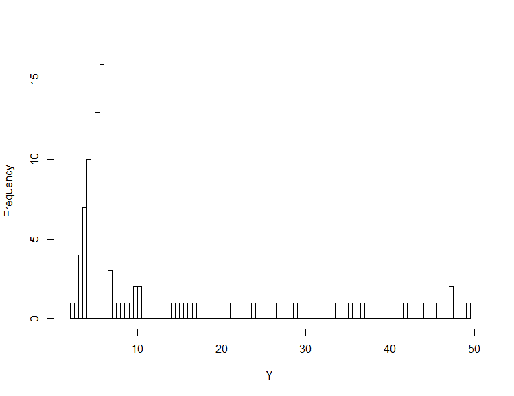
hist(Y, breaks=100)The code above, generates N <- 100 data points from a mixture with a uniform and a normal component. With a probability of alpha <- 0.3 we choose from the uniform distribution, with 1-alpha we choose from the normal distribution.
Below, you can see the histogram of the generated data. Visually, it’s quite clear, that two underlying processes were used to generate the data.
Next, we will formulate our Bayesian model in the language, that JAGS is able to understand. JAGS will take care of Gibbs sampling and adapt the hyperparameters during this process.
model <- "
model{
  for(i in 1:N){
    # Log density for the normal part:
    ld_comp[i, 1] <- logdensity.norm(Y[i], mu, tau)
    # Log density for the uniform part:
    ld_comp[i, 2] <- logdensity.unif(Y[i], lower, upper)

    # The latent class part using dcat:
    component_chosen[i] ~ dcat(probs)

    # Select one of these two densities and normalise with a Constant:
    density[i] <- exp(ld_comp[i, component_chosen[i]] - Constant)

    # Generate a likelihood for the MCMC sampler:
    Ones[i] ~ dbern(density[i])
  }
# ... the model continues hereExplanation:
For each of the 100 observations we made, the model first generates the density (in log scale) for both, the normal and the uniform component of the model (with hyperparameters mu, tau, lower and upper). Then, via the dcat function, the model decides in a probabilistic manner about which component to choose - and picks the associated density. Next comes a trick, that is useful to end up with the right (probabilistic) choice of the component. The model has to choose the density, that is most suitable to fit a series of ones from a bernoulli experiment with that density. In other words, the density has to be maximized by the model in order to fit best.
The “maximizing the density” trick will result in adaptation of the hyperparameters, such that the maximum likelihood for the One’s vector can be achieved. Clever, heh?
The following part of the model handles the prior distributions for the models hyperparameters:
# Priors for 2 parameters using a dirichlet distribution:
probs ~ ddirch(c(1,1))
lower ~ dnorm(0, 10^-6)
upper ~ dnorm(0, 10^-6)
mu ~ dnorm(0, 10^-6)
tau ~ dgamma(0.01, 0.01)

# Specify monitors, data and initial values using runjags:
#monitor# lower, upper, probs, mu, tau
#data# N, Y, Ones, Constant
#inits# lower, upper, mu, tau
}"Explanation:
The vector probs will store the probabilities alpha and 1-alpha. Its prior distribution follows a dirichlet distribution of order two.
A normal prior is put on the scalars lower, upper and mu, and a gamma prior is set for tau. The last part are instructions for run.jags, which parameters to monitor during sampling and where to take the data from.
As you can see, the input to JAGS is only the observed values (Y), as well as the number of observations (N), the vector of Ones and a constant (see below).
# Initial values to get the chains started:
lower <- min(Y)-10
upper <- max(Y)+10
mu <- 0
tau <- 0.01

Ones <- rep(1,N)

# The constant needs to be big enough to avoid any densities >1 but also small enough to calculate probabilities for observations of 1:
Constant <- 10

results <- run.jags(model, sample=10000, thin=1, n.chains = 3)
resultsExplanation:
Back in R, we have to guess initial values for the hyperparameters. The run.jags call starts the sampling by JAGS, using 1000 steps to adapt the model and 4000 steps to burn-in (defaults). After that, the model is run for 10000 iterations.
The results are given as a table (truncated):
| parameter | mean | SD | SSeff | autocorrelation |
|---|---|---|---|---|
| probs[1] | 0.68819 | 0.05 | 9726 | 0.035 |
| probs[2] | 0.31181 | 0.05 | 9726 | 0.035 |
| lower | 4.0893 | 2.7 | 1553 | 0.365 |
| upper | 50.992 | 1.6 | 5222 | 0.046 |
| mu | 4.9559 | 0.11 | 14504 | -0.0026 |
| tau | 1.2 | 0.24 | 7913 | 0.0329 |
Looking at the mean column, it seems that the model recovered the true parameters very well. Only the hyperparameter lower suffered from high autocorrelation and a small effective sample size. What those numbers mean will be explored in a upcoming post.
Acknowledgements:
- Matt Denwood, for his very valuable help with the JAGS model. Credits to him for the One’s trick and the subtraction of the constant.
- Elizabeth Garrett-Mayer, for her clear explanation on latent class models.
This post is a follow-up of a question at stackoverflow.com.
Subscribe via RSS